Assuming you have OpenFOAM version 6 with environment variables set, here is all you need to download, compile, and run sofcFoam.
cd <myChosenParentDirectory>
git clone git://git.code.sf.net/p/openfuelcell/git openfuelcell
cd openfuelcell
cd src
./Allwmake
cd ..
cd run/<caseDirectory> #coFlow, counterFlow, crossFlow, ...
make mesh
make srun
make view
The sofcFoam model is an OpenFOAM [1]application for the simulation of solid oxide fuel cells. It is a single-cell and multi-cell stack model being developed within the open source Multi-Scale Integrated Fuel Cell (MuSIC) project. This document describes how to obtain and use sofcFoam.
To make more sense of what follows, it may be useful to begin with a brief overview of the model. (A more detailed view will be provided later). The model simulates a four region fuel cell, as depicted schematically in Figure 1(a). Between two interconnects we find an air region, an electrolyte, and a fuel region. The model uses a computational domain for each of these regions, and one more global domain for the entire cell. Each domain supports its own fields. Pressure, momentum and species mass fractions, for example, are solved on the air and fuel domains, and temperature is solved on the global domain. Global and regional information is transferred back and forth via grid cell mappings that are established during mesh generation/splitting. Porous cathode and anode zones, shown in Figure 1(b), are incorporated into the air and fuel regions, respectively, using Darcy’s Law. Electrochemistry is assumed to occur on the electrode-electrolyte interfaces. The resulting electrochemical mass fluxes give rise to Dirichlet velocity conditions and Neumann mass-fraction conditions on the air and fuel boundaries interfacing the electrolyte.
After an initialization phase, the model enters an iteration loop as follows:
(a) |
(b) |
OpenFoam
The openFuelCell program is being developed with the open source C++ objected oriented software OpenFOAM, therefore it is necessary to have a working installation of OpenFOAM. At time of writing, OpenFuellCell has been tested and is known to work with the repository release of 2.1.x [2].
Some experience running OpenFOAM applications, as might be obtained from OpenFoam tutorials, will be helpful. Instructions for building OpenFOAM come with the download, and further assistance can be obtained from the discussion forum [3]. The WIKKI pages [4]are also useful for supplementary information.
Git
The sofcFoam code is maintained in a Git [5] version control system repository on SourceForge [6]. The Git command line client tool is git. Graphical tools are also available, e.g. , SmartGit [7].
A tar file containing the latest version of the OpenFuelCell code can be downloaded here from SourceForge [8].
Alternatively, users can check out the latest version of the code from the SourceForge git repository using the command...
git clone git://git.code.sf.net/p/openfuelcell/git openfuelcell
From Figure 2(a), the left panel of Figure 2, we see that the openfuelcell/ directory has two main subdirectories, run/ and src/. The run/ directory contains examples of cases that can be simulated with the model, while the src/ directory contains the model source code.
openfuelcell/run/
The run directory contains case directories, or cases. The cases coFlow, counterFlow, and crossFlow exercise the model on co-flow, counter-flow, and cross-flow configurations, respectively. The case quickTest is similar to the coFlow case, but reduced from twelve to three channels. The case quickTestStack is similar to quickTest but for a stack of three cells with external fuel and air manifolds. In each configuration, the fuel velocity is in the +x direction, while the air velocity is in the direction of +x, -x, and +y for co-flow, counter-flow and cross-flow, respectively.
openfuelcell/src/
The src/ directory contains the major subdirectories libSrc/ and appSrc/. In libSrc/, we find C++ classes that have been specifically developed or modified for sofcFoam and are used in the sofcFoam model. The appSrc/ directory contains the sofcFoam model source files, which instantiate objects from both libSrc/ and OpenFoam/src as needed, to implement the sofcFoam algorithm. As is typical for OpenFoam applications, the sofcFoam application is built by including blocks of code (*.H files) into a main program (*.C file).
run/
    coFlow/
        0/
            air/
            fuel/
        system/
            air/
            electrolyte/
            fuel/
            interconnect0/
            interconnect1/
        config/
        constant/
            polyMesh/
            air/
            electrolyte/
            fuel/
            interconnect0/
            interconnect1/
    counterFlow/
        <...like coFlow...>
    crossFlow/
        <...like coFlow...>
    quickTest/
        <...like coFlow...>
src/
    appSrc/
        Make/
    libSrc/
        continuityErrs/
        diffusivityModels/
            diffusivityModel/
            binaryFSG
            fixedDiffusivity/
            fsgDiffusionVolumes/
            fsgMolecularWeights/
            knudsen/
            porousFSG/
        Make/
        MeshWave/
        polyToddYoung/
        regionProperties/
        smearPatchToMesh/
        sofcSpecie/
|
0/ k T air/ p U YN2 YO2 fuel/ p U YH2 YH2O Allclean config/ make.faceAir make.faceFuel make.faceSet make.setAir make.setFuel make.setSet constant/ cellProperties rxnProerties air/ airProperties porousZones sofcSpeciesProperties electrolyte/ electrolyteProperties fuel/ fuelProperties porousZones sofcSpeciesProperties interconnect0/ interconnectProperties interconnect1/ interconnectProperties polyMesh/ blockMeshDict Makefile runscript system/ controlDict.mesh controlDict.run controlDict fvSchemes fvSolution decomposeParDict createPatchDict air/ fvSchemes fvSolution fuel/ fvSchemes fvSolution electrolyte/ fvSchemes fvSolution interconnect0/ fvSchemes fvSolution interconnect1/ fvSchemes fvSolution |
(a) | (b) |
Like any other OpenFoam case directory, the four cases here contain major subdirectories 0/, constant/, and system/. With only a single mesh, these 0/, constant/ and system/ directories would be populated by files only, but with multiple meshes they have a subdirectory for each region, and the files for each domain are placed in the appropriate directory or subdirectory. Thus initial global temperature T is found in 0/T, initial air velocity U in 0/air/U, initial fuel pressure p in 0/fuel/p, etc. Similarly, global cell properties are found in constant/cellProperties, whereas air properties are found in constant/air/airProperties. See Figure 2(b) for more complete listings.
In your chosen parent directory for the sofcFoam model, (e.g. your OpenFoam work space $WM_PROJECT_USER_DIR/applications/), check out the master branch, from the git repository [9] using your favourite graphical git tool, or the command
git clone git://git.code.sf.net/p/openfuelcell/git openfuelcell
This creates directory openfuelcell/ in the current working directory.
src
To compile the library and application source code, go to openfuelcell/src/ directory and run the Allwmake script. Type ./Allwmake at the prompt. This should generate shared object library libsofcFoam.so in the $FOAM_USER_LIBBIN directory and application executable sofcFoam in the $FOAM_USER_APPBIN directory. A lnInclude/ directory, containing links to all of the libSrc class files, will appear in the libSrc/ directory.
cases
As can be seen in Figure 2(b), a case directory contains only one polyMesh/ directory immediately after checkout, and it contains only the dictionary file blockMeshDict. This dictionary, together with the setSet batch command files in the <case>/config/ directory, describes the global and regional meshes. After the global mesh is made by the OpenFOAM utility blockMesh, the utility splitMeshRegions generates the required regional meshes and map files. For more information on the blockMesh, setSet, and setsToZones utilities, see Chapter 5 “Mesh generation and conversion [10]” and Section 3.6 “Standard utilities [11]” in the OpenFOAM User Guide [12].
Making the global and regional meshes is handled in sofcFoam by the Makefile in the case directory. See, for example, run/coFlow/Makefile. The command
make mesh
issued from the case directory, will generate the global mesh and the region meshes. During model execution, various material property and other field values will be mapped from the region meshes to the global mesh. Cells that began life labeled as a fluid in the global mesh may have become a solid, and some of these may have boundary faces on the original fluid inlet or outlet patches. Accordingly, the fluid inlet and outlet patches may need to be redefined for the new reality. The redefinitions are specified by the make.face[Air|Fuel|Set] files in the config directory. See Appendix A for a description of the steps required to specify a new geometry.
With the application compiled, the command:
make srun
will run the executable from the command line, using the available case data. The model can also be run by typing the executable name, and the output directed to Standard Out can be redirected to a file:
sofcFoam | tee log.run
Instead of running the model from the command line, a runscript is available to submit a job to a queue. The script usage line may need editing for your queuing system.
After the model has run to completion, VTK files for visualization, e.g. with paraview, can be prepared easily using the Makefile. Typing:
make view
will generate VTK files for the last output step, whereas:
make viewAll
will generate VTK files for all output directories.
Case quickTestPar is essentially case quickTest, modified for parallel decomposition. The makefile, however, is different from the serial file.
Edit system/decomposeParDict
Export environment variable NPROCS to desired number of processors (e.g. in csh: setenv NPROCS n)
make mesh
Builds the mesh
make parprep
Decompose the mesh and initial field data
make run
Run the decomposed case in parallel
make reconstruct
Reconstruct the mesh and data
make view
Generate the VTK files for viewing.
To start over type:
./Allclean
Here, the field files in the region subdirectories 0/air and 0/fuel have counterparts on the global mesh, i.e., in the top level of the 0/ directory. These files in the top level 0/ directory will be subset during parallel mesh splitting, and the subset fields will be moved to the processor/0/air and processor/0/fuel directories.
In the out−of−box case configuration, air species are O2 and N2, while fuel species are H2 and H2O. If species Sp are added or changed, it is necessary to have diffSp and YSp files for the new species, in accordance with sections 11.8.4 and 11.8.5 of the "gettingStarted_Cell268_OF21x.pdf" document in the docs/ directory. In order to reconstruct and visualize the fluid region fields, the fluid region polyMesh subdirectories must be present in the constant directory. Furthermore, the *ProcAddressing files usually generated by decomposePar −region <name> are required in the processor polyMesh directories.
We also need the *RegionAddressing files in our processor polyMesh directories to enable mapping between global and region meshes.
Accomplishing all of the above requires two decompositions for parallelism, one for the region meshes only and one for the entire mesh. The second decomposition can’t proceed in the presence of the processor* directories created from the first decomposition, so we rename them to keep their *ProcAddressing files for later use. There are also two mesh splittings, the second of them in parallel.
We proceed with steps 1 to 11 below. Note that Step 2 is controlled by the makefile:
$ make mesh | tee log.mesh
Steps 3 through 11 are controlled by parprep.csh, either directly or through the Makefile:
$ ./parprep.csh or $ make parpre
Step 10 is controlled by cleanup.csh, which contains lists noGlobal, noAir and noFuel, of files that are to be removed from, respectively, the processor*/0, processor*/0/air and processor*/0/fuel directories. These lists may need to be edited for additions or changes, particularly with respect to species. cleanup.csh is executed within parprep.csh.
To run the code:
mpirun −mca mpi_warn_on_fork 0 −np $NPROCS sofcFoam −parallel
The script
prun
will issue the above command, and
make runwill launch the prun script.
To reconstruct the parallel run:
reconstructPar
reconstructPar −region air
reconstructPar −region fuel
or simply
make reconstruct
To make the VTK files
foamToVTK −latestTime
foamToVTK −latestTime −region air
foamToVTK −latestTime −region fuel
foamToVTK −latestTime −region electrolyte
foamToVTK −latestTime −region interconnect0
foamToVTK −latestTime −region interconnect1
or simply
make view
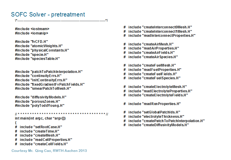
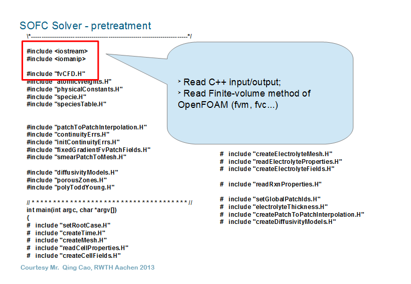
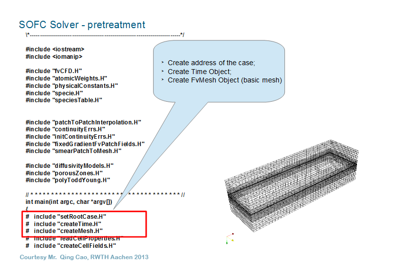
In this section, we will follow the main function, in the file sofcFoam.C, through the model execution. Like all OpenFOAM applications, the model begins by including the OpenFOAM src files setRootCase.H to check the case path, and createTime.H to read the system/controlDict file and instantiate the Time object runTime. This is followed by the creation of meshes, reading of properties, and creation of fields for the global cell mesh and the region meshes.
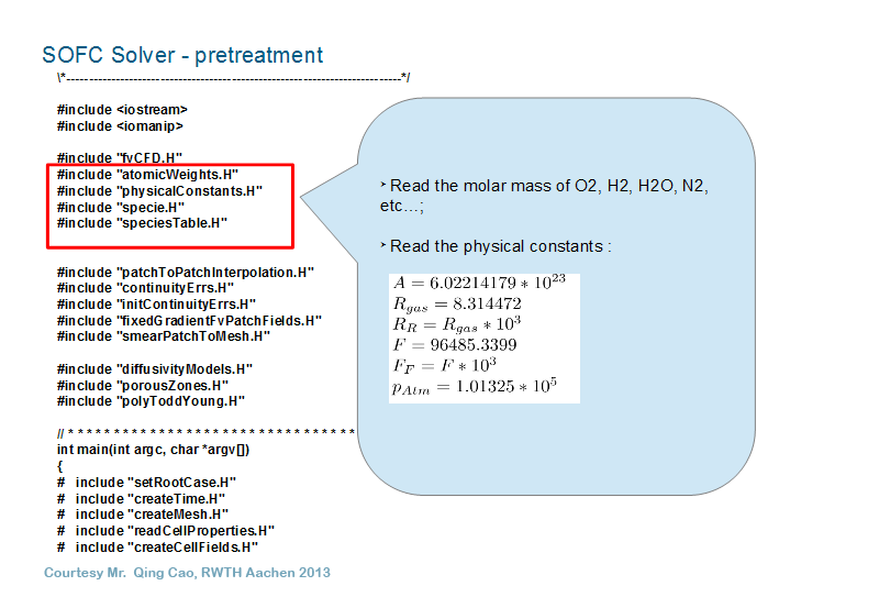
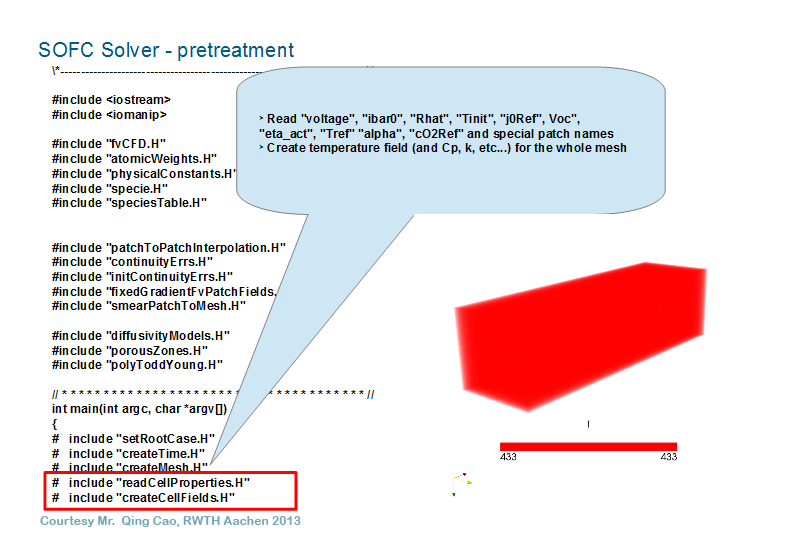
The first mesh to be created is the mesh for the entire cell. This is accomplished by the included file $FOAM_SRC/OpenFOAM/lnInclude/createMesh.H.. Mesh data is obtained from the constant/polyMesh directory. Global cell properties, or parameters, as listed in Table 1, above, are read from case file constant/cellProperties into model variables by appSrc file readCellProperties.H. Fields for the entire cell are created as IOobjects in appSrc file createCellFields.H. Some of the IOobjects have the MUST_READ attribute and must have a file in the starting time directory. The file name must be the same as the name specified in the IOobject. Others have the READ_IF_PRESENT attribute. The corresponding files will be read if they are present in the starting time directory. Still others have the NO_READ attribute and any file with their name will be ignored at field creation. Fields with IOobjects having the AUTO_WRITE attribute will write a file in the output time directories, whereas those with the NO_WRITE attribute aren’t written.
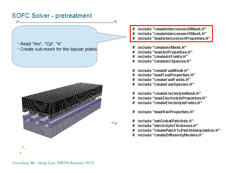
Similarly, meshes, properties, and fields are established for the regions interconnect0, air, electrolyte, fuel, and interconnect1. The meshes are created by the appSrc files create<Region>Mesh.H. These files specify the location of the region’s polyMesh directory and also create face-, cell-, and patch-maps to the global mesh. Constant properties are read by read<Region>Properties.H from case files constant/<region>/<region>Properties, and fields are read from case files 0/<region>/<fieldName> by appSrc file create<Region>Fields.H. Note that there are no fields on either of the interconnect meshes, and both interconnects are assumed to have the same properties.
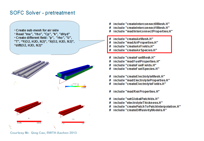
A number of air and fuel fields are specific to the species that comprise the fluid. The key appSrc files are createAirSpecies.H and createFuelSpecies.H. The key case files are constant/air/sofcSpeciesProperties and constant/fuel/sofcSpeciesProperties. See these for details of input data format.
As just indicated, the air species names and associated data are read from the constant/air/sofcSpeciesProperties file at run time by appSrc file createAirSpecies.H. A speciesTable object airSpeciesNames is instantiated from the list of species following the key word speciesList in the sofcSpeciesProperties file.
A pointerList, airSpecies, of pointers to sofcSpecie objects is created. The i-th air species can then be referenced as airSpecies[i]. For each specie in the air mixture, the specie properties of name, molar weight, molar charge (for Faraday’s law), reaction sign (produced=1, non-reacting=0, consumed=-1), enthalpy of formation, and standard entropy are stored in an sofcSpecie object, and can be accessed by class functions name(), MW(), ne(), rSign(), hForm() and sForm(), respectively. The sofcSpecie class can be found in src/libSrc.
After reading the species data, one of the species is designated as airInertSpecie. It is found after the keyword inertSofcSpecie in the sofcSpeciesProperties file. Note that the inertSpecie may well be chemically inert (non-reacting), but need not be. Here “inert” means that the mass fraction of the specie will not be computed from a partial differential equation, but rather calculated by adding the mass fractions of the other components and subtracting that sum from 1. The “inert” nomenclature follows that of OpenFOAM’s thermophysicalModels.
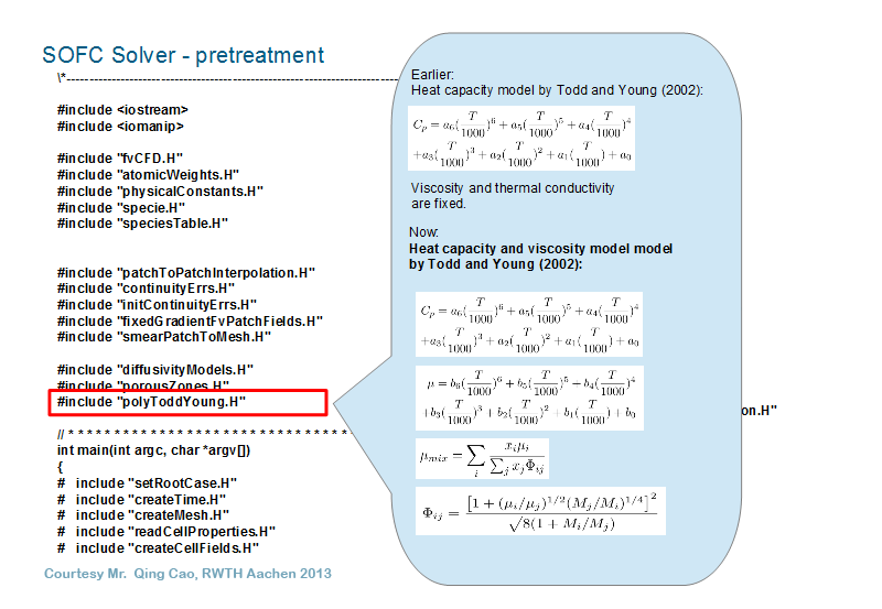
The sofcSpeciesProperties file concludes with a toddYoung dictionary of Todd-Young (2002) polynomial coefficients for molar isobaric heat capacity. These are used to create a pointerList, molarCpAir, of pointers to polyToddYoung objects. The polyToddYoung class has functions to evaluate the polynomial and to also evaluate definite integrals which correspond to enthalpy and entropy in the case of isobaric heat capacity (see src/libSrc/polyToddYoung). Thus, eg, we can evaluate the isobaric heat capacity of the i-th air species at ambient temperature with the expression molarCpAir[i].polyVal(Tair.internalField()).
The specie names are used to create a pointerList, Yair, to mass fraction fields with names of the form Ysp, where “sp” is one of the specie names. There is one such file for each specie in the mixture. The mass fraction field IOobjects are MUST_READ, so must exist as files in the starting time directory.
Mole fraction fields are calculated from the mass fraction fields. Their names have the form Xsp. The read/write attributes are NO_READ, AUTO_WRITE. Again we have a pointerList, Xair, so that Xair[i] references the mole fraction field of the i-th air species.
Finally, createAirSpecies.H establishes a pointerlist, diffSpAir, to scalar fields for the diffusivities of the individual species in the mixture. These have READ_IF_PRESENT and AUTO_WRITE attributes, and are created with initial value 1.
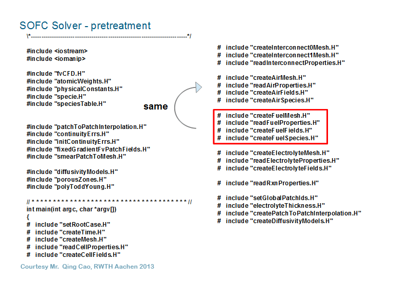
A completely analogous discussion applies to the fuel side.
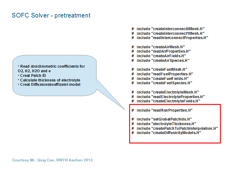
The chemical species involved in the reaction and their stoichiometric coefficients are listed after the rxnSpecies keyword in the constant/rxnProperties case file. The species “e” must always be in the list. Its coefficient is the number of moles of electrons transferred in the reaction. The list is read by appSrc file readRxnProperties.H, where a hash table, rxnSpCoef, is created. Thus a specie’s stoichiometric coefficient can be obtained via its name, e.g., rxnSpCoef["O2"], or rxnSpCoef[airSpecies[i].name()].
For convenience, global variables are established for the IDs (indices) of a number of patches that are frequently referenced. These patches were assigned to variable names in appSrc file readCellProperties.H, reading from case file constant/cellProperties. Their IDs are found and assigned in appSrc file setGlobalPatchIds.H.
Electrolyte thickness is used in the calculation of the electrolyte’s volumetric heat source term for the energy equation. It is calculated, in appSrc file electrolyteThickness.H, as the electrolyte volume divided by the average area of the anode and cathode interfaces. Average area is used to take into account cylindrical cells.
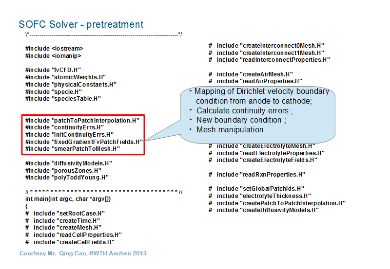
Electrochemistry is assumed to occur within the electrolyte. Mole fraction patch fields of oxidants on the air side (cathode) interface and of hydrogen and water on the fuel side (anode) must be therefore interpolated to fields in the electrolyte. The resulting current density is calculated on the fuel side of the anode interface and must be interpolated to the electrolyte side in order to calculate the electrolyte’s volumetric heat source terms. These interpolations are carried out by OpenFOAM patchToPatchInterpolation objects, created in appSrc file createPatchToPatchInterpolation.H.
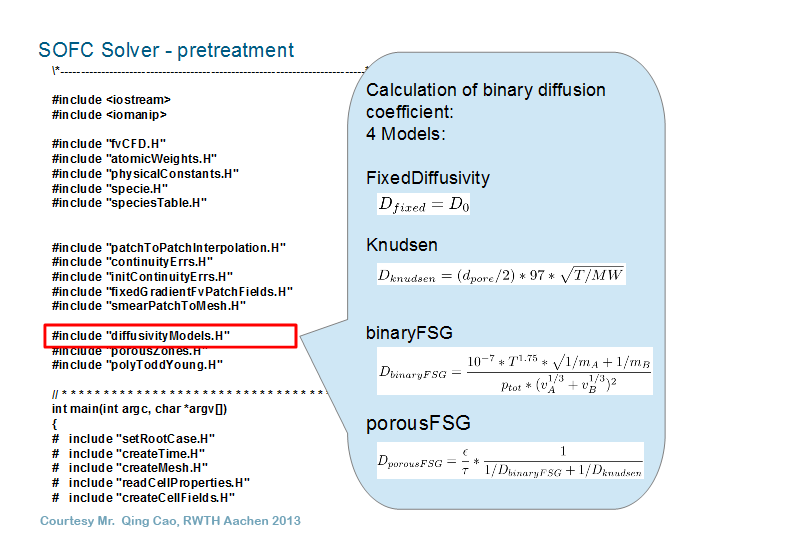
The diffusivity models are created in appSrc file createDiffusivityModels.H. For both air and fuel, a pointerList of diffusivity models is declared. On the air side, this is airDiffModels. Creation of a new diffusivity model requires a scalar field for the calculated diffusivity values, a label list of cells for which the diffusivity is to be calculated (normally corresponding to a cell zone), and a dictionary specifying the model type along with the corresponding type-specific parameters.
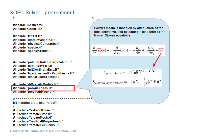
On the air side, a scalarField, airDiff, is used by each airDiffusivityModel[m] to return its calculated values. Then, a diffusivity model is established for each air zone and a pointer to it is added to the pointerList. There is one model for the entire air zone. Its dictionary is located in the constant/air/airProperties case file. There is also one model for each porous zone within the air region, with dictionaries in the corresponding zone in the case file constant/air/porousZones. The cellZone labelLists are found in the polyMesh directory for the air region.
An analogous story holds on the fuel side. How the SOFC model uses the diffusivity models will be described below.
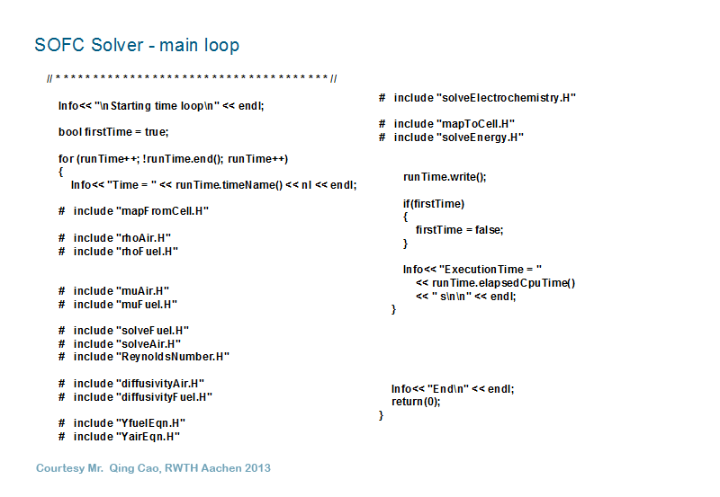
A number of calculations are repeated until convergence.
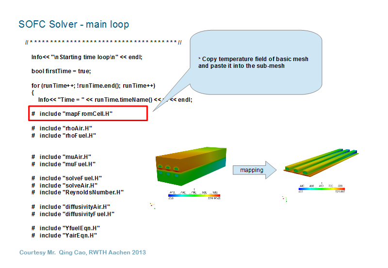
The fluid regions need local temperature fields in order to calculate local fluid density. The mapping is done in appSrc file mapFromCell.H, using the cell maps established during mesh creation.
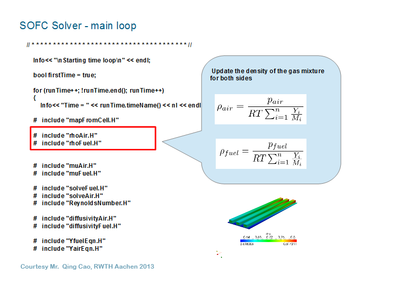
Fluid densities ρ are calculated from pressure p, temperature T, constituent mass fractions yi and molar weights Mi as
$$\rho =\frac{p}{RT\mathop{\sum }^{}\left( {{y}_{i}}/{{M}_{i}} \right)}$$
where R is the universal gas constant. The calculations are coded in appSrc files rhoAir.H and rhoFuel.H.
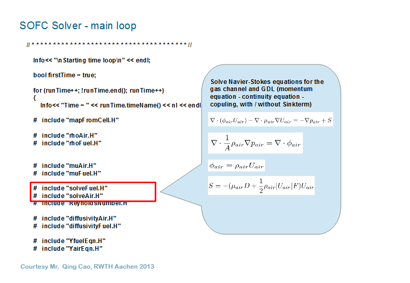
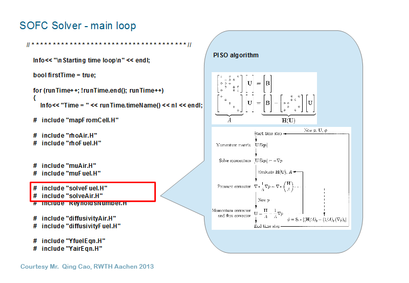
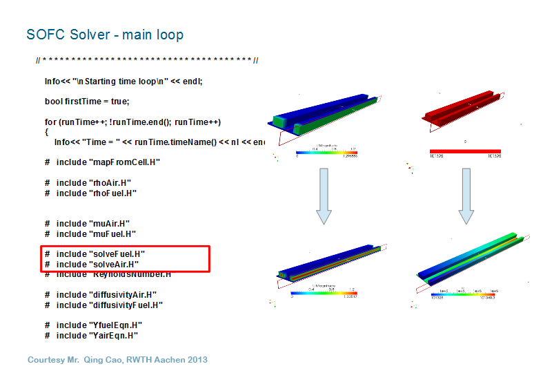
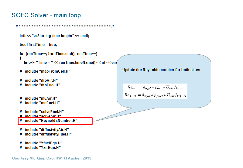
Pressure and momentum are solved using the PISO iteration in appSrc files solveAir.H and solveFuel.H. Following the solution, the Reynolds numbers are calculated in appSrc file ReynoldsNumber.H. These are informative only, and require the input of hydraulic diameter of the gas channels, in case files constant/air/airProperties and constant/fuel/fuelProperties.
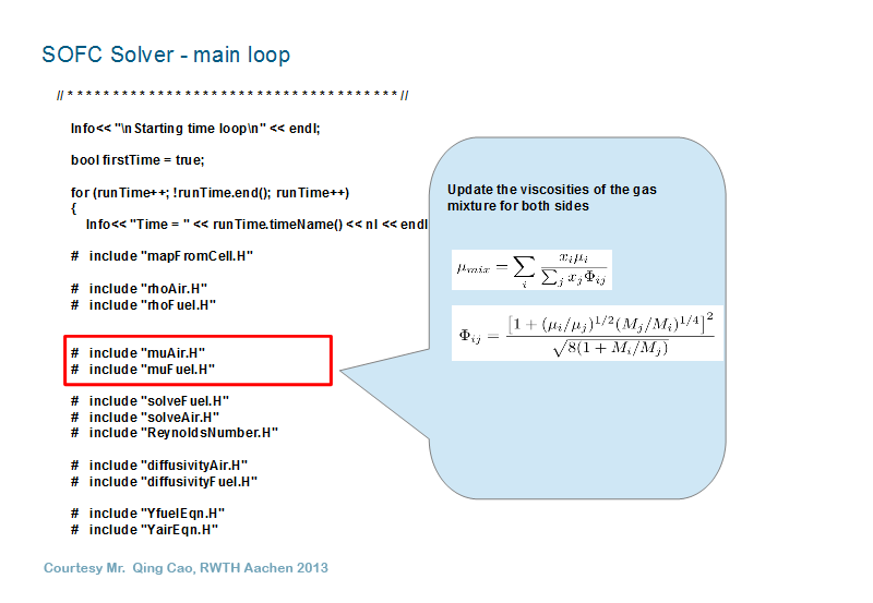
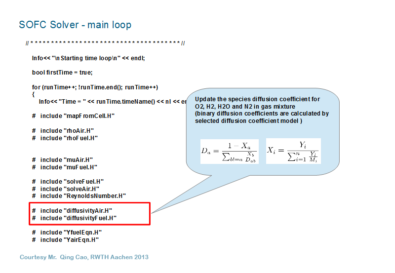
The diffusivities are calculated in appSrc files diffusivityAir.H and diffusivityFuel.H. The following discussion refers only to air, but applies equally to fuel. Of interest is the diffusivity, D(a), of specie a in the mixture. A diffusivity field is thus calculated for each specie, except for the background “inert” specie. A specie a can be given a fixed diffusivity value using the fixedDiffusivity model, or its diffusivity in the mixture, D(a), can be modelled from the pairwise binary diffusivities D(a,b) of specie a diffusing in specie b.
The sofcFoam model combines pairwise binary diffusivities following Wilke (1950):
$$D\left( a \right)=~\frac{1-~{{x}_{a}}}{{{S}_{a}}}$$
where
$${{S}_{a}}~=\underset{b\ne a}{\mathop \sum }\,\frac{{{x}_{b}}}{D\left( a,b \right)}$$
with mole fractions x and specie indices a,b.
The calculation proceeds by first fixing specie a, stepping through the species b and accumulating the results to obtain the sum Sa, which is then used to get D(a). The computed diffusivity is stored in volScalarField diffSpAir[a].
The diffusivity calculations have the following algorithmic structure:
forAll(airSpecies, a)
{
  if(airSpecies[a].name() != airInertSpecie)
  {
    forAll(airDiffModels, m)
    {
      if(airDiffModels[m]->isFixed())
      {
        //obtain fixed diffusivity
      }
      else if(!airDiffModels[m]->isBinary())
      {
         Error: must have fixed or binary: exit
      }
      else
      {
        initialize sumA = 0
        forAll(airSpecies,b)
        {
          if (b != a)
          {
            set specie b in airDiffModel[m]
            calculate binary diffusivity
            accumulate sumA
          }
        }
          obtain diffusivity in mixture using sumA
        } //isBinary
      } //m
    } //!inert
  } //a
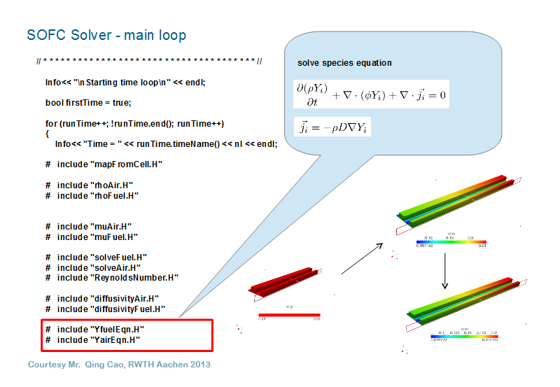
Mass fractions are computed in appSrc files YairEqn.H and YfuelEqn.H. For each specie other than the background “inert” specie, a partial differential equation is solved for Yair[i], where i is the specie index. The mass fraction of the “inert” specie is obtained by subtracting the sum of all the other species’ mass fractions from 1.
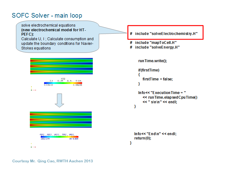
Electrochemistry is assumed assumed to occur on the anode interface with the electrolyte. It is calculated in appSrc file solveElectrochemistry.H. Global temperature is interpolated to the fuel mesh anode patch. Reactant oxidant species mole fractions are computed on the air mesh cathode patch and interpolated to the fuel mesh anode patch. Reactant and product fuel species are also calculated on the fuel mesh anode patch.
With all fields defined on the anode patch, the mole fractions, temperature, and specie properties are used to calculate the Nernst potential, E, via included appSrc file NernstEqn.H. Area specific resistance, R, is modelled by a function in included appSrc file ASRfunction.H. Current density i is then calculated as
$$i=\frac{E-V-\eta}{R}$$
where V and \(\eta\) are the present values of voltage and activation overpotential. The voltage is subsequently corrected using the present and prescribed mean current densities.
Electrochemical heating is calculated in included appSrc file electrochemicalHeating.H. Specie enthalpies are calculated and combined with enthalpy of formation and Joule heating in the electrolyte volume.
Species electrochemical mass fluxes are calculated and used to set Neumann boundary conditions on the cathode and anode patches for the calculation of air and fuel mass fractions, and Dirichlet conditions for the air and fuel velocities.
For the reaction
$$\text{rxn:}\ \ \sum\limits_{i}{{}}{{a}_{i~}}{{R}_{i~}}=~\underset{j}{\mathop \sum }\,{{b}_{j}}{{P}_{j}}$$
having reactants Ri with stoichiometric coefficients ai and products Pj with stoichiometric coefficients bj, the Nernst potential, E, is calculated as
$$E=~{{E}_{0}}-~\frac{RT}{zF}\text{ln}Q$$
where R is the universal gas constant, F is Faraday’s constant, z is the number [moles] of electrons transferred,
$$Q=~\frac{\mathop{\prod }_{j}{{\left[ {{P}_{j}} \right]}^{{{b}_{j}}}}}{\mathop{\prod }_{i}{{\left[ {{R}_{i}} \right]}^{{{a}_{i}}}}}$$
with [ denoting mole fraction, and
$${{E}_{0}}=~-\frac{\Delta {{G}_{\text{rxn }\!\!~\!\!\text{ }\!\!~\!\!\text{ }}}}{F}=~-\frac{\left( \Delta {{H}_{\text{rxn}}}-T\Delta {{S}_{\text{rxn}}} \right)}{F}$$
where
$$\Delta {{H}_{\text{rxn}}}~=~\underset{j}{\mathop \sum }\,{{b}_{j}}\Delta H\left( {{P}_{j}} \right)-\underset{i}{\mathop \sum }\,{{a}_{i}}\Delta H({{R}_{i}})$$
and
$$\Delta {{S}_{\text{rxn}}}~=~\underset{j}{\mathop \sum }\,{{b}_{j}}\Delta S\left( {{P}_{j}} \right)-\underset{i}{\mathop \sum }\,{{a}_{i}}\Delta S({{R}_{i}})$$
For species X,
$$\Delta H\left( X \right)=~\underset{{{T}_{0}}}{\overset{T}{\mathop \int }}\,{{C}_{p,X}}\left( T \right)dT$$
and,
$$\Delta S\left( X \right)=~\underset{{{T}_{0}}}{\overset{T}{\mathop \int }}\,\frac{{{C}_{p,X}}\left( T \right)dT}{T}$$
where T0 and T are reference and ambient temperatures, respectively. Todd-Young polynomials for molar heat capacity are used to evaluate the and integrals, using polyToddYoung class functions polyInt and polyIntS, respectively.
The cell activation overpotential is presumed to be composed of anodic and cathodic contributions: \[\eta ={{\eta }_{a}}+{{\eta }_{c}}\] Defining the electrode overpotential, \({{\eta }_{e}}={{\eta }_{a}}\) at the anode and \({{\eta }_{e}}={{\eta }_{c}}\) at the cathode. Values of \({{\eta }_{e}}\left( i \right)\) at both electrodes are obtained using a root finder based on Ridder's method coded in appSrc file, riddersRoot.C, to obtain numerical solutions of the Butler-Volmer equation \[{i}={{{i}}_{0}}\left[ \exp \left( A{{\eta }_{e}} \right)-\exp \left( B{{\eta }_{e}} \right) \right]\] where \[{A=2{{\alpha }_{e}}F}/{RT}\;\]\[{B=-2\left( 1-{{\alpha }_{e}} \right)F}/{RT}\;\] at each electrode. The exchange current densities are given by; \[{{{i}}_{0,c}}={{\gamma }_{c}}p_{{{\text{O}}_{2}}}^{m}\exp \left( -\frac{{{E}_{act,c}}}{RT} \right)\] \[{{{i}}_{0,a}}={{\gamma }_{a}}p_{{{\text{H}}_{2}}}^{a}p_{{{\text{H}}_{\text{2}}}\text{O}}^{b}\exp \left( -\frac{{{E}_{act,a}}}{RT} \right)\]
The reaction orders, a, b, m, the pre-constants \({{\gamma }_{a}}\), \({{\gamma }_{c}}\), activation energies Eact,a , Eact,c are prescribed together with the transfer coefficients, \({{\alpha }_{e}}\), \({{\alpha }_{c}}\) in the dictionary activationParameters, located in constant/electrolyte. The prescibed values are those recommended in Leonide at el. (2009). Note the partial pressures are in Atmospheres.
Heating sources for the energy solution are comprised of enthalpy of reactions (assumed to occur on the electrolyte/fuel interface), enthalpy changes of gaseous species from reference to ambient temperature, and resistive heating. It is assumed that there is no reaction on the air side. The volumetric source terms are ascribed to the electrolyte region.
Enthalpy of formation and enthalpy changes, normalized by number of contributing electrons, are calaculated by specie, accumulating products and reactants separately for each of air and fuel. The separate (normalized) enthalpy accumulations are then combined according to
\[{{h}_{src}}=\left( {{h}_{form}}+{{h}_{P,fuel}}-{{h}_{R,fuel}}+{{h}_{P,air}}-{{h}_{R,air}} \right)\frac{i}{F{{l}_{e}}}\]
where i is current density, F is Faraday’s constant, le is the electrolyte thickness, hform is accumulated enthalpy of formation, hP,fuel is accumulated enthalpy change of products on the fuel side, hR,fuel is accumulated enthalpy change of reactants on the fuel side, and similarly for the air side. The final source for the energy equation then becomes
$${{S}_{\text{energy}}}=-{{h}_{\text{src}}}-\frac{iV}{{{l}_{e}}}$$
An electrochemical mass flux is calculated for each specie taking part in the reaction, in accordance with Faraday’s law, and taking into account whether the specie is consumed or produced:
$${{\dot{m}}^{''}}=~\pm \frac{Mi}{\nu F}$$
where M is molar mass, i is current density, ν is valence, and F is Faraday’s constant. Air species are treated separately from fuel species, and separate sums of air and fuel fluxes are accumulated for later use. The plus sign is used for products and the negative sign for reactants. On the air side, the above calculations are coded at lines 164 to 177 of solveElectrochemistry.H.
Mass fractions Y of all species, except the background “inert” specie, are found by solving a partial differential equation. Mass is transferred through the electrode boundaries, so these boundary fields are cast to a fixedGradient type, to which a (generally non-uniform) gradient value is assigned. The mass fraction gradient of a specie i will be due to both mass flux of i and to the mass fluxes of the other species. Letting Yi be the mass fraction boundary field of specie i on the electrode boundary, we have
$$\frac{\partial {{Y}_{i}}}{\partial n}={1\over{\rho D}}\left(\dot{m}_{i}^{''}\left( 1-{{Y}_{i~}} \right)-{{Y}_{i}}\underset{j\ne i}{\mathop \sum }\,\dot{m}_{j}^{''}\right)$$
The mass flux sums are used to calculate Dirichlet velocity boundary conditions for air on the cathode and for fuel on the anode. Note that the calculations take place with fields defined on the anode interface, so patchToPatchInterpolation to the air side is required. Then, we have for U on the boundary
\[{{\left. \mathbf{U} \right|}_{\text{electrode}~\text{ }}}=-\frac{\sum{{{\dot{m}}''}}}{\rho }\frac{\mathbf{A}}{\left\| \mathbf{A} \right\|}~\]
where \(\mathop{\sum }^{}{{\dot{m}}^{''}}\) is the accumulated mass flux, ρ is the fluid density, and \({{\mathbf{A}}/{\left\| \mathbf{A} \right\|}\;}\) is the unit outward normal.
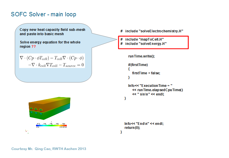
In order to solve the energy equation, regional values of thermal conductivity, heat capacity, density, velocity, etc., are required on the global mesh. Prior to any mapping, the internal values of the recipient fields on the global mesh are reset to zero by appSrc file mapToCell.H. Regional fields are then mapped to the global mesh by appSrc files map<Region>ToCell.H for each of the regions air, fuel, electrolyte, interconnect0 and interconnect1.
In the case of the solids, there is no convective heat transfer, so velocity and heat capacity for the corresponding space within the global mesh will simply be set to zero. Density and thermal conductivity are assumed uniform and are given by the values in their properties files. In the case of the electrolyte, the volumetric energy source terms computed there are also mapped to a global energy source field.
For the fluids, we have both convective and diffusive heat transfer. Mass based heat capacity of the mixture, cp, is calculated as a linear combination of the specie molar heat capacities, Cp,i, divided by their molar mass, Mi, using mass fraction, Yi, as the linear coefficients:
$${{c}_{p}}=\underset{i}{\mathop \sum }\,\frac{{{Y}_{i}}{{C}_{p,i}}}{{{M}_{i}}}$$
Thermal conductivity is assumed to be uniform within each fluid zone. In the fluid channels it takes the value read from the fluid properties file, whereas in the porous zones it is a linear combination of the channel value and the porous zone value weighted by porosity. Porosity and porous zone thermal conductivity are obtained from the porous zone dictionary.
Rather than mapping velocity directly, it is the fluxes \(\phi =\rho \mathbf{U}\centerdot \mathbf{dA}\) (computed during the pressure-velocity calculation such that mass conservation is satisfied) that are required for the finite volume equations. The fluxes form a surface field on the mesh faces and are mapped onto the global faces corresponding to the regional meshes interior faces and also to the regional mesh boundary patches. At this stage, we have fluxes on the fluid sides of the fluid/electrolyte interfaces, but not on the electrolyte side, the electrolyte being a solid. This can result in heat leaving or entering a fluid through its boundary with the electrolyte, without a corresponding gain or loss within the electrolyte. This situation is remedied by zeroing all fluxes that touch the electrolyte and introducing an additional compensating source term into the energy equation. The zeroing of fluxes is done in mapElectrolyteToCell.H. The source term is equivalent to the continuity error introduced by the zeroing of the fluxes on the electrolyte boundaries.
After the regional fields are mapped to the corresponding locations in the global mesh, the global energy is computed from a partial differential equation in appSrc file solveEnergy.H. The equation is essentially
\[\operatorname{div}\left( \rho \mathbf{U}{{c}_{p}}T \right)-{{S}_{\phi }}-\operatorname{div}\left( k\operatorname{grad}T \right)={{S}_{q}}\]
where \({{S}_{q}}\) is a volumetric heat source and \({{S}_{\phi }}\) is the source due to the zeroed fluxes on the electrolyte boundary faces. The term \(-{{S}_{\phi }}\) appears in the discrete equation as
fvm::SuSp(-fvc::div(rhoCpPhiCell), Tcell)
where rhoCpPhiCell is equal to the face interpolated cp multiplied by the surface scalar field phiCell. Note that phi already incorporates rho. The finite volume matrix operator SuSp linearizes the source term and adds the linear part to the matrix diagonal or to the source in such a way as to maximize diagonal dominance of the matrix.
Figure A1 shows the proposed geometry we intend to model. The associated dimensions of the components are given in Table A1. The vertical structure can be captured by seven blocks, as shown in Figure A2, (the block containing the electrolyte is too thin to be discernible). The blocks containing the air and fuel channels can then be split horizontally to separate the channels from the ribs, the latter being part of the interconnects.
 |  |  |
| Figure A1. A fuel cell with one air channel and one fuel channel. Left panel shows air (blue) and fuel (purple) inlets, interconnects (grey) and electrode sides. Centre panel shows air (blue) and fuel (purple) volume regions, each comprised of both a channel and a porous electrode zone. Right panel shows lower (blue) and upper (red) interconnect regions. | ||
| interconnect0 | air channel | cathode | electrolyte | anode | fuel channel | interconnect1 | |
|---|---|---|---|---|---|---|---|
| xlow | 0 | 0 | 0 | 0 | 0 | 0 | 0 |
| xhigh | 50 | 50 | 50 | 50 | 50 | 50 | 50 |
| length [mm] | 50 | 50 | 50 | 50 | 50 | 50 | 50 |
| ylow | 0 | 1 | 0 | 0 | 0 | 1 | 0 |
| yhigh | 4 | 3 | 4 | 4 | 4 | 3 | 4 |
| width [mm] | 4 | 2 | 4 | 4 | 4 | 2 | 4 |
| zlow | 0 | 3.5 | 5.00 | 5.29 | 5.3 | 6.3 | 6.3 |
| zhigh | 5 | 5.0 | 5.29 | 5.30 | 6.3 | 7.8 | 11.3 |
| height [mm] | 5 | 1.5 | 0.29 | 0.01 | 1 | 1.5 | 5 |
|
| Bottom to top: interconnect0, air, cathode, electrolyte (too thin to discern), anode, fuel, and interconnect1. |
We begin with a blockMeshDict dictionary that will create a parent mesh consisting of the seven vertical blocks (Figure A2), which for convenience, going from bottom to top, we refer to as interconnect0, air, cathode, electrolyte, anode, fuel, and interconnect1. Although the geometry shows symmetry about the y = 2 plane, we construct the entire domain for illustrative purposes. Here is the list of points for the blockMeshDict file:
blockMeshDictIn the vertices section above, each set of four vertices defines a horizontal rectangle representing an interface between the above mentioned blocks (and including the top and bottom surfaces). As can be readily seen, the vertices of a rectangle are arranged so that a traversal from one to the next takes one anticlockwise around the rectangle, starting from x=0. Note that the coordinates are scaled by 0.001 metres, so the maximum x-coordinate, for example, is 50 mm. The vertices are numbered by their index in the list, beginning at index 0. Figure A3 shows the location of some of these points on the geometry.
convertToMeters 0.001;
vertices
(
// ... From Bottom To Top
// Interconnect0
( 0 0 0) // 0
(50 0 0) // 1
(50 4 0) // 2
( 0 4 0) // 3
// Interconnect0_to_Air
( 0 0 3.5) // 4
(50 0 3.5) // 5
(50 4 3.5) // 6
( 0 4 3.5) // 7
// Air_to_cathode
( 0 0 5.0) // 8
(50 0 5.0) // 9
(50 4 5.0) //10
( 0 4 5.0) //11
// cathode_to_Electrolyte
( 0 0 5.29) //12
(50 0 5.29) //13
(50 4 5.29) //14
( 0 4 5.29) //15
// Electrolyte_to_anode
( 0 0 5.3) //16
(50 0 5.3) //17
(50 4 5.3) //18
( 0 4 5.3) //19
// anode_to_Fuel
( 0 0 6.3) //20
(50 0 6.3) //21
(50 4 6.3) //22
( 0 4 6.3) //23
// fuel_to_Interconnect1
( 0 0 7.8) //24
(50 0 7.8) //25
(50 4 7.8) //26
( 0 4 7.8) //27
// Interconnect1
( 0 0 11.3) //28
(50 0 11.3) //29
(50 4 11.3) //30
( 0 4 11.3) //31
);
 |
In the blocks section below, each hexahedral block is defined by two successive sets of four vertices, i.e. the corner vertices of the block. The air block, eg, is defined by: hex (4 5 6 7 8 9 10 11). The number of cells in each coordinate direction and the grading of the mesh are also prescribed here.
blocksWe have no need to define any edges.
(
// Interconnect0
hex (0 1 2 3 4 5 6 7) (25 8 7) simpleGrading (1 1 1)
// air
hex (4 5 6 7 8 9 10 11) (25 8 3) simpleGrading (1 1 1)
// cathode
hex (8 9 10 11 12 13 14 15) (25 8 1) simpleGrading (1 1 1)
// electrolyte
hex (12 13 14 15 16 17 18 19) (25 8 1) simpleGrading (1 1 1)
// anode
hex (16 17 18 19 20 21 22 23) (25 8 2) simpleGrading (1 1 1)
// fuel
hex (20 21 22 23 24 25 26 27) (25 8 3) simpleGrading (1 1 1)
// Interconnect1
hex (24 25 26 27 28 29 30 31) (25 8 7) simpleGrading (1 1 1)
);edges
(
);
A patch consists of one or more outer boundaries of the blocks. These boundaries (rectangles in our case) are described by their corner vertices, arranged so that a traversal from one to the next takes one round the rectangle anticlockwise about the outward normal.
patches
(
// ... From Bottom to Top
// Interconnect0
patch interconnect0Bottom
(
(0 3 2 1)
)
patch interconnect0Sides
(
(0 1 5 4)
(3 7 6 2)
(0 4 7 3)
(1 2 6 5)
)
// Air
patch airInlet
(
(4 8 11 7)
)
patch airOutlet
(
(5 6 10 9)
)
patch airSides
(
(4 5 9 8)
(7 11 10 6)
)
// Cathode
patch cathodeSides
(
(8 9 13 12)
(11 15 14 10)
(8 12 15 11)
(9 10 14 13)
)
// Electrolyte
patch electrolyteSides
(
(12 13 17 16)
(15 19 18 14)
(12 16 19 15)
(13 14 18 17)
)
// Anode
patch anodeSides
(
(16 17 21 20)
(19 23 22 18)
(16 20 23 19)
(17 18 22 21)
)
// Fuel
patch fuelInlet
(
(20 24 27 23)
)
patch fuelOutlet
(
(21 22 26 25)
)
patch fuelSides
(
(20 21 25 24)
(23 27 26 22)
)
// interconnect1
patch interconnect1Sides
(
(24 28 31 27)
(25 26 30 29)
(24 25 29 28)
(27 31 30 26)
)
patch interconnect1Top
(
(28 29 30 31)
)
);
mergePatchPairs
(
);
// **********************************
For more description of the blockMeshDict dictionary and the blockMesh utility, see section 5.3, Mesh generation with the blockMesh utility, in the OpenFoam User Guide [13].
We must now define the cellSets that will make up the cells of our five regions: interconnect0, air, electrolyte, fuel and interconnect1. Using the cellSets, a mesh will be generated for each region. Note that the cathode and anode blocks will become porousZones within the air and fuel regions, respectively. A portion of the air block contains two ribs that must become part of the interconnect0 region, and similarly two ribs contained in the fuel block must become part of the interconnect1 region. Cells in the electrolyte block will form the electrolyte region, and cells in the interconnect blocks will become part of the interconnect regions.
The cellSets for the regions are specified in config/make.setSet. Here each cellSet is defined by the diagonally opposite corners of a box bounded by coordinate planes.
The first set specified is the cellSet interconnect0. The specification begins with the cells in the interconnect0 block, which consists of all the cells below z=3.5mm (note that the coordinates are given in metres). Then the cells of the ribs are added. One of these extends from y=0 mm to y=1 mm, and the other from y=3 mm to y=4 mm. Both extend the full length of 50 mm in x, and in height from z=3.5 mm to z=5 mm.
The specification for the air cellSet begins with the cathode block and adds the channel, which extends the full length of 50 mm in x, from y=1 mm to y=3 mm in width, and from y=3.5 mm to y=5 mm in height. The remaining sets are similarly specified.
make.setSet
cellSet interconnect0 new boxToCell (0 0.0e-3 0.0e-3) (50.0e-3 4.0e-3 3.5e-3)
cellSet interconnect0 add boxToCell (0 0.0e-3 3.5e-3) (50.0e-3 1.0e-3 5.0e-3)
cellSet interconnect0 add boxToCell (0 3.0e-3 3.5e-3) (50.0e-3 4.0e-3 5.0e-3)
cellSet air new boxToCell (0 0.0e-3 5.0e-3) (50.0e-3 4.0e-3 5.29e-3)
cellSet air add boxToCell (0 1.0e-3 3.5e-3) (50.0e-3 3.0e-3 5.0e-3)
cellSet electrolyte new boxToCell (0 0 5.29e-3) (50.0e-3 4.0e-3 5.3e-3)
cellSet fuel new boxToCell (0 0.0e-3 5.3e-3) (50.0e-3 4.0e-3 6.3e-3)
cellSet fuel add boxToCell (0 1.0e-3 6.3e-3) (50.0e-3 3.0e-3 7.8e-3)
cellSet interconnect1 new boxToCell (0 0.0e-3 7.8e-3) (50.0e-3 4.0e-3 11.3e-3)
cellSet interconnect1 add boxToCell (0 0.0e-3 6.3e-3) (50.0e-3 1.0e-3 7.8e-3)
cellSet interconnect1 add boxToCell (0 3.0e-3 6.3e-3) (50.0e-3 4.0e-3 7.8e-3)
The air and fuel regions are each given a porous zone within the fluid zone, as specified in config/make.setAir and config/make.set fuel:
make.setAir
cellSet air new boxToCell (0 0.0e-3 5.0e-3) (50.0e-3 4.0e-3 5.29e-3)
cellSet air add boxToCell (0 1.0e-3 3.5e-3) (50.0e-3 3.0e-3 5.0e-3)
cellSet cathode new boxToCell (0 0 5.0e-3) (40.0e-3 4.0e-3 5.29e-3)
make.setFuel
cellSet fuel new boxToCell (0 0.0e-3 5.3e-3) (50.0e-3 4.0e-3 6.3e-3)
cellSet fuel add boxToCell (0 1.0e-3 6.3e-3) (50.0e-3 3.0e-3 7.8e-3)
cellSet anode new boxToCell (0 0 5.3e-3) (50.0e-3 4.0e-3 6.3e-3)
Clearly, the fluid inlet and outlet patches on the global mesh are incorrect, since their original definitions include faces that are really part of the interconnect ribs. The correction proceeds in three steps. First, faceSets for all of the existing patches of the blockMesh are created using the patchToFace action of the faceSet utility, as specified by the config/make.faceSet file:
faceSet interconnect0Sides new patchToFace interconnect0Sides allNote that the make.faceset file also specifies some manipulations, adding faceSets airInlet, airOutlet, and airSides to the faceSet interconnect0, and similary on the fuel side. After being added, they are subsequently cleared. Next, the inlet and outlet faceSets are corrected using new specifications in config/make.faceAir and config/make.faceFuel:
faceSet interconnect0Bottom new patchToFace interconnect0Bottom all
faceSet interconnect1Sides new patchToFace interconnect1sides all
faceSet interconnect1Top new patchToFace interconnect1Top all
faceSet electrolyteSides new patchToFace electrolyteSides all
faceSet cathodeSides new patchToFace cathodeSides all
faceSet airSides new patchToFace airSides all
faceSet airInlet new patchToFace airInlet all
faceSet airOutlet new patchToFace airOutlet all
faceSet anodeSides new patchToFace anodeSides all
faceSet fuelSides new patchToFace fuelSides all
faceSet fuelInlet new patchToFace fuelInlet all
faceSet fuelOutlet new patchToFace fuelOutlet all
faceSet interconnect0Sides add patchToFace airInlet all
faceSet interconnect0Sides add patchToFace airOutlet all
faceSet interconnect0Sides add patchToFace airSides all
faceSet interconnect1Sides add patchToFace fuelInlet all
faceSet interconnect1Sides add patchToFace fuelOutlet all
faceSet interconnect1Sides add patchToFace fuelSides all
faceSet airSides clear
faceSet airInlet clear
faceSet airOutlet clear
faceSet fuelSides clear
faceSet fuelInlet clear
faceSet fuelOutlet clear
make.faceAir
faceSet airInlet new boxToFace (-1e-6 1.0e-3 3.5e-3) (1e-6 3.0e-3 5.0e-3)
faceSet airOutlet new boxToFace (39.999e-3 1.0e-3 3.5e-3) (40.001e-3 3.0e-3 5.0e-3)
faceSet interconnect0Sides delete faceToFace airInlet all
faceSet interconnect0Sides delete faceToFace airOutlet all
make.faceFuel
faceSet fuelInlet new boxToFace (-1e-6 1e-3 6.3e-3) (1e-6 3.0e-3 7.8e-3)
faceSet fuelOutlet new boxToFace (39.999e-3 1e-3 6.3e-3) (40.001e-3 3.0e-3 7.8e-3)
faceSet interconnect1Sides delete faceToFace fuelInlet all
faceSet interconnect1Sides delete faceToFace fuelOutlet all
The new inlet and outlet patches are defined by a bounding box for the new patch. Here the new airInlet, eg, is normal to the x-direction and is bounded by a box which is shallow in x, extending 1e-6 m in front of and behind the prescribed x-coordinate location. The lateral extents of the box in the other two directions correspond to the lateral extent of the inlet in those directions. Faces with face centre within the box will be selected, so the box must not extend to the adjacent grid cell. The fuelInlet and the two outlets are similarly defined. The new inlets and outlets are then removed from the interconnect faceSets.
Finally, the faceSets are used to create new patches using the createPatch utility, which is controlled by the system/createPatchDict file. Here is an excerpt for the airInlet patch:
patchInfo
(
{
name airInlet;
// Type of new patch
dictionary
{
type patch;
}
constructFrom set;
patches ();
set airInlet;
}
. . .
);
We will find the following entry (with additional face numbering information) for the airInlet in the mesh boundary file.airInlet
{
type patch;
}
The remaining patches are formed in the same way. The complete patch list is:interconnect0Bottom
interconnect0Sides
airInlet
airOutlet
cathodeSides
electrolyteSides
anodeSides
fuelInlet
fuelOutlet
interconnect1Sides
interconnect1Top
Links
[1] http://www.openfoam.com/
[2] http://www.openfoam.org/archive/2.1.0/download/git.php
[3] http://www.cfd-online.com/Forums/openfoam
[4] http://openfoamwiki.net/index.php/Main_Page
[5] http://git-scm.com
[6] http://sourceforge.net/openfuelcell/git
[7] http://www.syntevo.com/smartgit/index.html
[8] https://sourceforge.net/projects/openfuelcell/files/
[9] https://sourceforge.net/p/openfuelcell/git/
[10] http://www.openfoam.org/docs/user/mesh.php#x22-1270005
[11] http://www.openfoam.org/docs/user/standard-utilities.php#x14-900003.6
[12] http://www.openfoam.org/docs/user/
[13] http://www.openfoam.org/docs/